AE and VAE on Fashion-MNIST

Overview

                Autoencoders (AE) and Variational Autoencoders (VAE) compared on Fashion-MNIST (70,000 images,
                10 classes). Both compress 784-dimensional images into a low-dimensional latent space.
                Key findings: AE achieves lower reconstruction error (MSE 0.032 at dim 32); VAE produces
                a structured latent space enabling reliable generative sampling.
            

0.032

AE Best Test MSE (dim 32)

28.4

VAE Best ELBO (dim 32)

dim 32

Best Latent Dimension

5×10⁻⁴

Optimal Learning Rate

Architecture

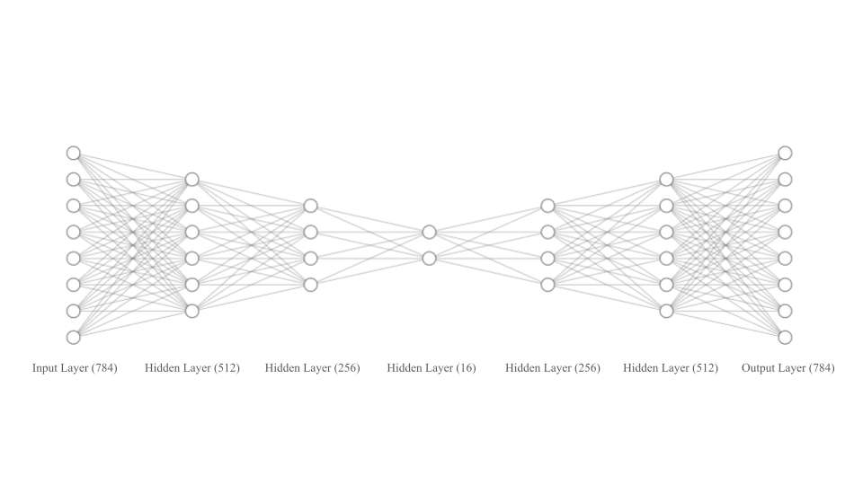
Figure 1: Autoencoder (AE) and Variational Autoencoder (VAE) architecture diagram

Autoencoder (AE)

Encoder: 784 → 512 → 256 → z (ReLU)
Decoder: z → 256 → 512 → 784 (Tanh)
Encoder outputs a single fixed vector z
Loss: MSE reconstruction

Variational Autoencoder (VAE)

Same encoder-decoder backbone
Encoder outputs μ and log σ² (two parallel heads)
Sample z = μ + ε·σ (reparameterization trick)
Loss: MSE + KL divergence (β=1)

Both models use Adam optimizer, mini-batch size 128, 30 epochs. Images normalized to [−1, 1] to match Tanh output. Training set (60,000) split 90/10 into train (54,000) and validation (6,000); test set (10,000) held out.

Results

Loss Curves

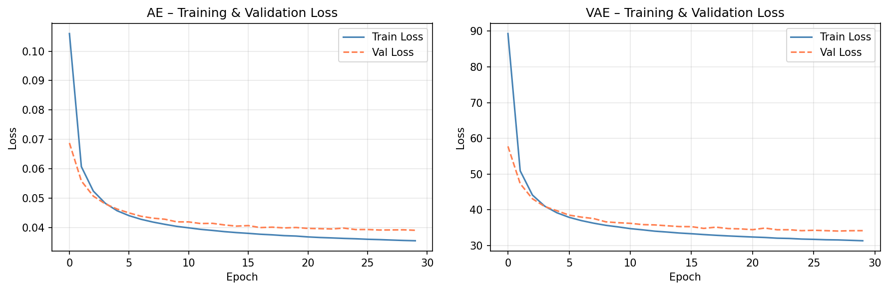
Figure 2: Training and Validation loss over 30 epochs — AE (left) and VAE (right) at baseline (dim=16, lr=1×10⁻³)

Both models converge smoothly with no overfitting. At baseline: AE test MSE = 0.039, VAE test ELBO = 34.23. These values are not directly comparable since the VAE's ELBO includes the KL term.

Reconstructions

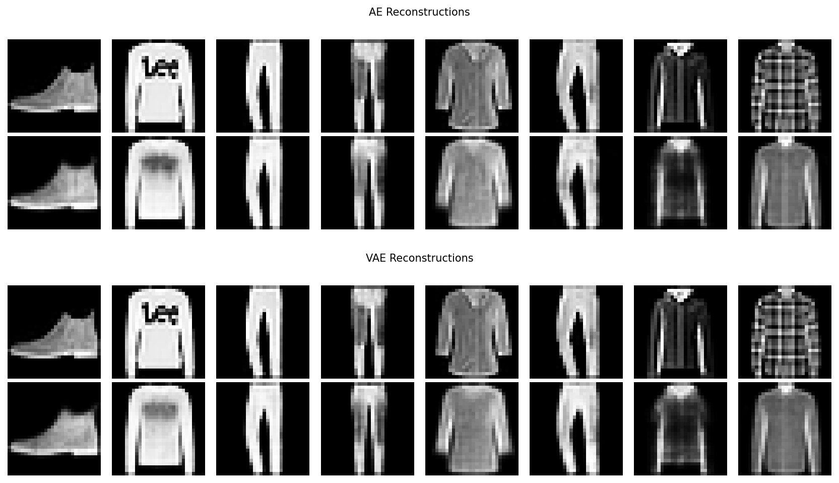
Figure 3: Original images (upper row) and reconstructions (lower row) within each panel — AE above, VAE below

Both models recover the overall shape and class of each garment. AE outputs are slightly sharper; VAE outputs are mildly smoother due to the KL penalty spreading the latent posterior.

Hyperparameter Analysis — Latent Dimension & Learning Rate

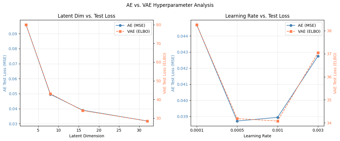
Figure 4: Test Loss vs. Latent Dimension (left) and Test Loss vs. Learning Rate (right)

Latent Dim	AE Test MSE	VAE ELBO
2	0.097	79.9
8	0.050	43.0
16	0.039	34.6
32	0.032	28.4

The largest gain occurs between dim 2 and 8; gains diminish beyond 16. Optimal learning rate: 5×10⁻⁴–1×10⁻³ (under-converged at 1×10⁻⁴, overshoots at 3×10⁻³).

Latent Space Visualization (t-SNE)

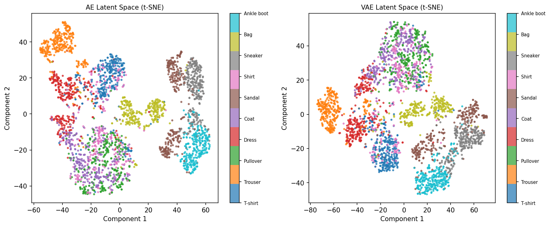
Figure 5: t-SNE of 3,000 test encodings — AE latent space (left) and VAE latent space (right)

The AE latent space is fragmented — class clusters overlap with empty voids between them. The VAE latent space is denser and more organized, with cleaner class separation due to KL regularization.

VAE Generated Samples

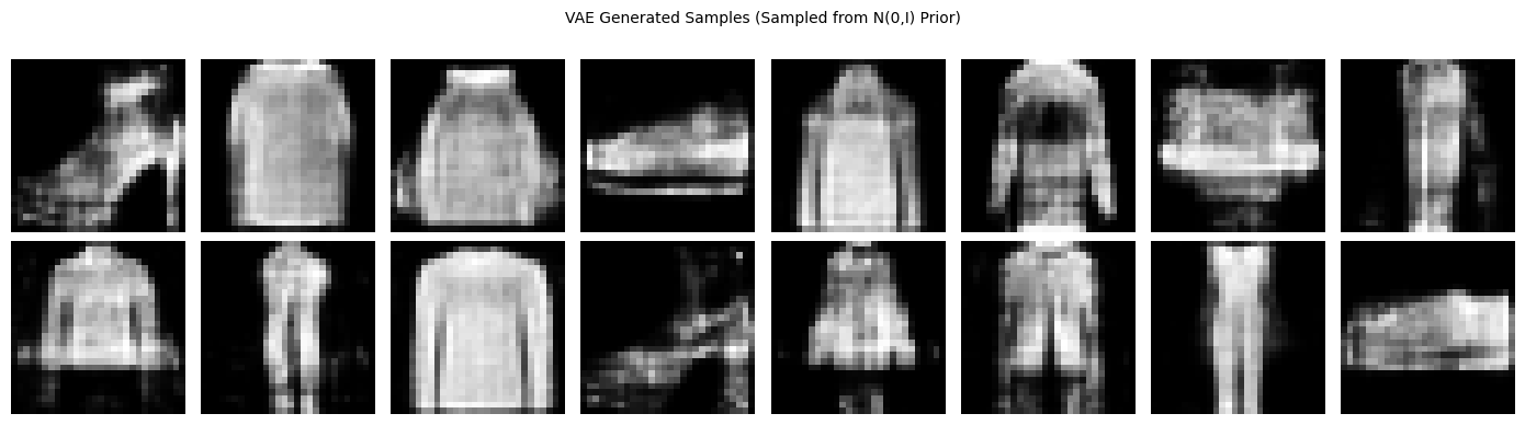
Figure 6: 16 samples generated by the VAE from N(0,I) prior — visually coherent clothing silhouettes

The VAE's structured prior supports reliable generation. Sampling z~N(0,I) produces plausible clothing images, confirming the continuous, well-organized latent space. The AE cannot do this — its unstructured latent space does not guarantee valid decodings between training points.

Conclusion

The AE achieved lower reconstruction error (MSE 0.032 at dim 32) due to unconstrained optimization — preferable for discriminative tasks.
The VAE's KL regularization produced a smoother, more organized latent space that enables reliable generation — essential for generative tasks.
Best latent dimension was 32, though gains beyond 16 were diminishing.
Optimal learning rate range: 5×10⁻⁴–1×10⁻³ — consistent for both models.
Future work: convolutional encoders, β-VAE, or conditional generation.

Dimensionality Reduction and Generative Modeling with Autoencoders and Variational Autoencoders on Fashion-MNIST